Foreword

Recently, I was studying a paper “Mining Quality Phrases from Massive Text Corpora”, which talked about how to mine high-quality phrases from massive text corpora, which used the Random Forest (Random Forest) algorithm, so I went to study it. Before I blogged It has been explained specifically for Decision Tree. Random Forest is an optimized version based on Decision Tree. Let’s discuss what Random Forest is.

1. What is Random Forest?

As a highly flexible machine learning algorithm, Random Forest (RF) has a wide range of application prospects, from marketing to health care insurance, it can be used for marketing simulation modeling, customer source statistics, retention and loss, can also be used to predict disease risk and susceptibility of patients. In domestic and foreign competitions in recent years, including the 2013 Baidu Campus Movie Recommendation System Competition, the 2014 Alibaba Tianchi Big Data Competition and the Kaggle Data Science Competition, participants used random forests in a very high proportion. So it can be seen that Random Forest still has a considerable advantage in terms of accuracy.

Having said so much, what kind of algorithm is random forest?

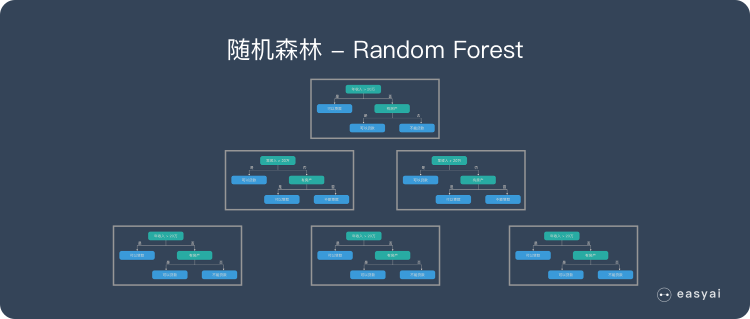
If readers have been exposed to decision trees (Decision Tree), then it will be easy to understand what is a random forest. Random forest is an algorithm that integrates multiple trees through the idea of ensemble learning. Its basic unit is a decision tree, and its essence belongs to a large branch of machine learning – the ensemble learning method. There are two keywords in the name of random forest, one is “random” and the other is “forest”. We understand “forest” very well. If one tree is called a tree, then hundreds or thousands of trees can be called a forest. This metaphor is very appropriate. In fact, this is also the main idea of random forest – the embodiment of integration thinking. The meaning of “random” will be discussed in the next section.

In fact, from an intuitive point of view, each decision tree is a classifier (assuming that it is now targeting a classification problem), then for an input sample, N trees will have N classification results. The random forest integrates all the classification voting results, and designates the category with the most votes as the final output. This is the simplest Bagging idea.

Random Forest is a powerful and versatile supervised machine learning algorithm that grows and combines multiple decision trees to create a “forest”. It can be used for classification and regression problems in R and Python.

Before we explore random forests in more detail, let’s break it down:

What is supervised learning?
What are classification and regression?
What is a decision tree?
Understanding each of these concepts will help you understand random forests and how they work. So let’s explain.

1.1 What is supervised machine learning?

A function (model parameters) is learned from a given training data set, and when new data arrives, results can be predicted based on this function. The training set requirements for supervised learning include input and output, which can also be said to be features and targets. Objects in the training set are annotated by humans. Supervised learning is the most common classification (attention and clustering distinction) problem. An optimal model (this model belongs to a set of functions, The optimal means that it is the best under a certain evaluation criterion), and then use this model to map all the inputs to the corresponding outputs, and make simple judgments on the outputs to achieve the purpose of classification. It also has the ability to classify unknown data. The goal of supervised learning is often to let the computer learn the classification system (model) that we have created.

Supervised learning is a common technique for training neural networks and decision trees. These two techniques highly rely on the information given by the pre-determined classification system. For neural networks, the classification system uses the information to judge the error of the network, and then continuously adjusts the network parameters. With decision trees, classification systems use it to determine which attributes provide the most information. Typical examples in supervised learning are KNN and SVM.

1.2 What are regression and classification?

In machine learning, algorithms are used to classify certain observations, events, or inputs into groups. For example, a spam filter will classify every email as “spam” or “not spam.” However, the email example is just a simple example; in a business setting, the predictive power of these models can have a significant impact on how decisions are made and how strategies are formed, but more on that later.

So: both regression and classification are supervised machine learning problems that are used to predict an outcome or the value or class of an outcome. Their difference is:

Classification problems are used to put a label on things, usually the result is a discrete value. For example, to judge whether the animal in a picture is a cat or a dog, classification is usually based on regression, and the last layer of classification usually uses the softmax function to judge its category. Classification does not have the concept of approximation, and there is only one correct result in the end, and the wrong one is wrong, and there will be no similar concept. The most common classification method is logistic regression, or logistic classification.

Regression problems are usually used to predict a value, such as predicting housing prices, future weather conditions, etc. For example, the actual price of a product is 500 yuan, and the predicted value through regression analysis is 499 yuan. We think this is a relatively good regression analysis . A more common regression algorithm is the linear regression algorithm (LR). In addition, regression analysis is used on the neural network, and the top layer does not need to add the softmax function, but directly accumulates the previous layer. Regression is an approximate prediction of the true value.

A simple way to distinguish between the two can be roughly stated that classification is about predicting labels (such as “spam” or “not spam”), while regression is about predicting quantities.

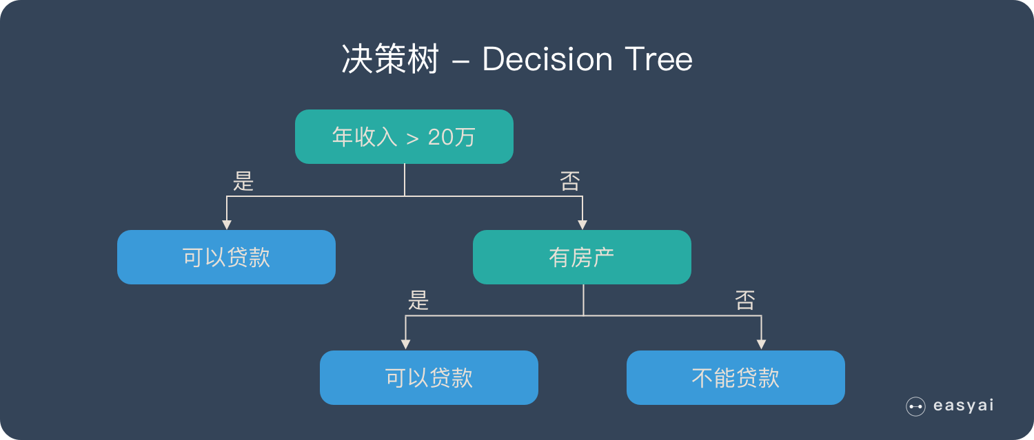
1.3 What is a decision tree?

Before explaining random forests, we need to mention decision trees. Decision tree is a very simple algorithm, which is highly explanatory and conforms to human intuitive thinking. This is a supervised learning algorithm based on if-then-else rules. The above picture can intuitively express the logic of the decision tree.

The derivation process of the decision tree is described in detail in my previous blog

Machine Learning – Decision Tree (1)

Machine Learning – Derivation of Decision Trees

1.4 What is Random Forest?

A random forest is composed of many decision trees, and there is no correlation between different decision trees.

When we perform a classification task, when a new input sample enters, each decision tree in the forest is judged and classified separately. Each decision tree will get its own classification result, which classification in the classification result of the decision tree At most, then Random Forest will take this result as the final result.

2. The construction process of Random Forest

2.1 Algorithm implementation

A sample with a sample size of N is drawn N times with replacement, one sample is drawn each time, and finally N samples are formed. The selected N samples are used to train a decision tree as samples at the root node of the decision tree.
When each sample has M attributes, when each node of the decision tree needs to be split, m attributes are randomly selected from the M attributes, satisfying the condition m << M. Then use a certain strategy (for example, information gain) from these m attributes to select 1 attribute as the splitting attribute of the node.
In the process of forming the decision tree, each node must be split according to step 2 (it is easy to understand, if the attribute selected by the node next time is the attribute used when its parent node was just split, the node has reached the leaf node, there is no need to continue to split), until it can no longer be split. Note that no pruning is performed throughout the formation of the decision tree.
Follow steps 1-3 to build a large number of decision trees, thus forming a random forest.

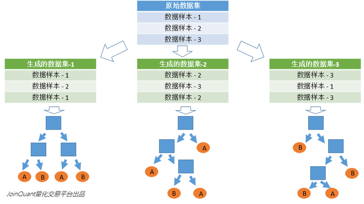
2.2 Random selection of data

First, sampling with replacement is taken from the original data set to construct a sub-data set, and the data volume of the sub-data set is the same as that of the original data set. Elements in different sub-datasets can be repeated, and elements in the same sub-dataset can also be repeated. Second, use sub-datasets to build sub-decision trees, put this data into each sub-decision tree, and each sub-decision tree outputs a result. Finally, if you have new data and need to obtain classification results through random forest, you can get the output of random forest by voting on the judgment results of the sub-decision tree. As shown in Figure 3, assuming that there are 3 sub-decision trees in the random forest, the classification result of 2 sub-trees is class A, and the classification result of 1 sub-tree is class B, then the classification result of random forest is class A.

2.3 Random selection of features to be selected

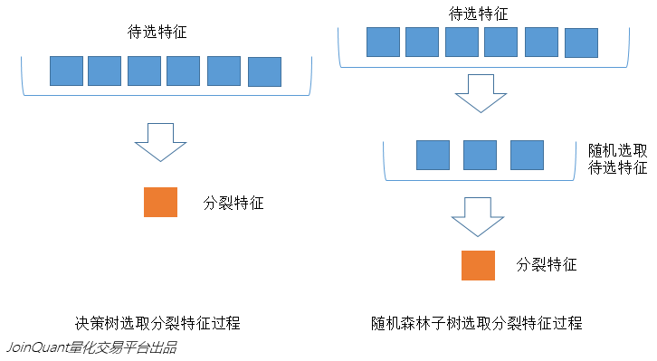
Similar to the random selection of the data set, each splitting process of the subtree in the random forest does not use all the features to be selected, but randomly selects certain features from all the features to be selected, and then randomly selects Select the best features among the features. In this way, the decision trees in the random forest can be different from each other, improving the diversity of the system, thereby improving the classification performance.

In the figure below, the blue squares represent all the features that can be selected, that is, the features to be selected. Yellow squares are split features. On the left is the feature selection process of a decision tree. By selecting the optimal split feature among the features to be selected (don’t forget the ID3 algorithm mentioned above, the C4.5 algorithm, the CART algorithm, etc.), the split is completed. On the right is the feature selection process for a subtree in a random forest.

2.4 Explanation of related concepts

1. Splitting: During the training process of the decision tree, it is necessary to split the training data set into two sub-data sets again and again. This process is called splitting.

2. Features: In classification problems, the data input to the classifier is called features. Taking the above stock price prediction problem as an example, the feature is the trading volume and closing price of the previous day.

3. Feature to be selected: In the process of constructing the decision tree, it is necessary to select features from all the features in a certain order. Candidate features are the set of features that have not been selected before the step. For example, all the features are ABCDE. In the first step, the feature to be selected is ABCDE. If C is selected in the first step, then in the second step, the feature to be selected is ABDE.

4. Split feature: The definition of the selected feature is received. The feature selected each time is the split feature. For example, in the above example, the split feature of the first step is C. Because these selected features divide the data set into disjoint parts, they are called split features.

3. Advantages and disadvantages of Random Forest

3.1 Advantages
It can produce very high-dimensional (many features) data without dimensionality reduction or feature selection
It can judge the importance of features
Interactions between different features can be judged
Not easy to overfit
The training speed is relatively fast, and it is easy to make a parallel method
It is relatively simple to implement
For unbalanced datasets, it balances the errors.
Accuracy can still be maintained if a large fraction of features are missing.

3.2 Disadvantages
Random forests have been shown to overfit on some noisy classification or regression problems
For data with attributes of different values, attributes with more value divisions will have a greater impact on random forests, so the attribute weights produced by random forests on such data are not credible
Since Random Forest uses many decision trees, it can require a lot of memory on larger projects. This can make it slower than some other more efficient algorithms
Four, Extra-Trees (extreme random tree)
The ET or Extra-Trees (Extremely randomized trees) algorithm is very similar to the random forest algorithm, consisting of many decision trees. The main difference between extreme trees and random forests:

1. randomForest applies the Bagging model, all the samples used by extraTree, but the features are randomly selected, because the split is random, so it is better than the results obtained by random forest to some extent

2. Random forest is to obtain the best bifurcation attribute in a random subset, and ET is to obtain the bifurcation value completely randomly, so as to realize the bifurcation of the decision tree

5. Python Implementation of Random Forest

5.1 Dataset
Network disk link: https://pan.baidu.com/s/1PK2Ipbsdx1Gy5naFgiwEeA
Extract code: t3u1

5.2 Python Implementation of Random Forest
# -*- coding: utf-8 -*-
import csv
from random import seed
from random import randrange
from math import sqrt

def loadCSV(filename):#加载数据，一行行的存入列表
dataSet = []
with open(filename, ‘r’) as file:
csvReader = csv.reader(file)
for line in csvReader:
dataSet.append(line)
return dataSet

# 除了标签列，其他列都转换为float类型
def column_to_float(dataSet):
featLen = len(dataSet[0]) – 1
for data in dataSet:
for column in range(featLen):
data[column] = float(data[column].strip())

# 将数据集随机分成N块，方便交叉验证，其中一块是测试集，其他四块是训练集
def spiltDataSet(dataSet, n_folds):
fold_size = int(len(dataSet) / n_folds)
dataSet_copy = list(dataSet)
dataSet_spilt = []
for i in range(n_folds):
fold = []
while len(fold) < fold_size: # 这里不能用if，if只是在第一次判断时起作用，while执行循环，直到条件不成立
index = randrange(len(dataSet_copy))
fold.append(dataSet_copy.pop(index)) # pop() 函数用于移除列表中的一个元素（默认最后一个元素），并且返回该元素的值。
dataSet_spilt.append(fold)
return dataSet_spilt

# 构造数据子集
def get_subsample(dataSet, ratio):
subdataSet = []
lenSubdata = round(len(dataSet) * ratio)#返回浮点数
while len(subdataSet) < lenSubdata:
index = randrange(len(dataSet) – 1)
subdataSet.append(dataSet[index])
# print len(subdataSet)
return subdataSet

# 分割数据集
def data_spilt(dataSet, index, value):
left = []
right = []
for row in dataSet:
if row[index] < value:
left.append(row)
else:
right.append(row)
return left, right

# 计算分割代价
def spilt_loss(left, right, class_values):
loss = 0.0
for class_value in class_values:
left_size = len(left)
if left_size != 0: # 防止除数为零
prop = [row[-1] for row in left].count(class_value) / float(left_size)
loss += (prop * (1.0 – prop))
right_size = len(right)
if right_size != 0:
prop = [row[-1] for row in right].count(class_value) / float(right_size)
loss += (prop * (1.0 – prop))
return loss

# 选取任意的n个特征，在这n个特征中，选取分割时的最优特征
def get_best_spilt(dataSet, n_features):
features = []
class_values = list(set(row[-1] for row in dataSet))
b_index, b_value, b_loss, b_left, b_right = 999, 999, 999, None, None
while len(features) < n_features:
index = randrange(len(dataSet[0]) – 1)
if index not in features:
features.append(index)
# print ‘features:’,features
for index in features:#找到列的最适合做节点的索引，（损失最小）
for row in dataSet:
left, right = data_spilt(dataSet, index, row[index])#以它为节点的，左右分支
loss = spilt_loss(left, right, class_values)
if loss < b_loss:#寻找最小分割代价
b_index, b_value, b_loss, b_left, b_right = index, row[index], loss, left, right
# print b_loss
# print type(b_index)
return {‘index’: b_index, ‘value’: b_value, ‘left’: b_left, ‘right’: b_right}

# 决定输出标签
def decide_label(data):
output = [row[-1] for row in data]
return max(set(output), key=output.count)

# 子分割，不断地构建叶节点的过程
def sub_spilt(root, n_features, max_depth, min_size, depth):
left = root[‘left’]
# print left
right = root[‘right’]
del (root[‘left’])
del (root[‘right’])
# print depth
if not left or not right:
root[‘left’] = root[‘right’] = decide_label(left + right)
# print ‘testing’
return
if depth > max_depth:
root[‘left’] = decide_label(left)
root[‘right’] = decide_label(right)
return
if len(left) < min_size:
root[‘left’] = decide_label(left)
else:
root[‘left’] = get_best_spilt(left, n_features)
# print ‘testing_left’
sub_spilt(root[‘left’], n_features, max_depth, min_size, depth + 1)
if len(right) < min_size:
root[‘right’] = decide_label(right)
else:
root[‘right’] = get_best_spilt(right, n_features)
# print ‘testing_right’
sub_spilt(root[‘right’], n_features, max_depth, min_size, depth + 1)

# 构造决策树
def build_tree(dataSet, n_features, max_depth, min_size):
root = get_best_spilt(dataSet, n_features)
sub_spilt(root, n_features, max_depth, min_size, 1)
return root
# 预测测试集结果
def predict(tree, row):
predictions = []
if row[tree[‘index’]] < tree[‘value’]:
if isinstance(tree[‘left’], dict):
return predict(tree[‘left’], row)
else:
return tree[‘left’]
else:
if isinstance(tree[‘right’], dict):
return predict(tree[‘right’], row)
else:
return tree[‘right’]
# predictions=set(predictions)
def bagging_predict(trees, row):
predictions = [predict(tree, row) for tree in trees]
return max(set(predictions), key=predictions.count)
# 创建随机森林
def random_forest(train, test, ratio, n_feature, max_depth, min_size, n_trees):
trees = []
for i in range(n_trees):
train = get_subsample(train, ratio)#从切割的数据集中选取子集
tree = build_tree(train, n_features, max_depth, min_size)
# print ‘tree %d: ‘%i,tree
trees.append(tree)
# predict_values = [predict(trees,row) for row in test]
predict_values = [bagging_predict(trees, row) for row in test]
return predict_values
# 计算准确率
def accuracy(predict_values, actual):
correct = 0
for i in range(len(actual)):
if actual[i] == predict_values[i]:
correct += 1
return correct / float(len(actual))

if __name__ == ‘__main__’:
seed(1)
dataSet = loadCSV(‘D:/深度之眼/sonar-all-data.csv’)
column_to_float(dataSet)#dataSet
n_folds = 5
max_depth = 15
min_size = 1
ratio = 1.0
# n_features=sqrt(len(dataSet)-1)
n_features = 15
n_trees = 10
folds = spiltDataSet(dataSet, n_folds)#先是切割数据集
scores = []
for fold in folds:
train_set = folds[
:] # 此处不能简单地用train_set=folds，这样用属于引用,那么当train_set的值改变的时候，folds的值也会改变，所以要用复制的形式。（L[:]）能够复制序列，D.copy() 能够复制字典，list能够生成拷贝 list(L)
train_set.remove(fold)#选好训练集
# print len(folds)
train_set = sum(train_set, []) # 将多个fold列表组合成一个train_set列表
# print len(train_set)
test_set = []
for row in fold:
row_copy = list(row)
row_copy[-1] = None
test_set.append(row_copy)
# for row in test_set:
# print row[-1]
actual = [row[-1] for row in fold]
predict_values = random_forest(train_set, test_set, ratio, n_features, max_depth, min_size, n_trees)
accur = accuracy(predict_values, actual)
scores.append(accur)
print (‘Trees is %d’ % n_trees)
print (‘scores:%s’ % scores)
print (‘mean score:%s’ % (sum(scores) / float(len(scores))))

5.3 Comparison of Decision Tree, Random Forest and Extra-Trees

# -*- coding: utf-8 -*-
from sklearn.model_selection import cross_val_score
from sklearn.datasets import make_blobs
from sklearn.ensemble import RandomForestClassifier
from sklearn.ensemble import ExtraTreesClassifier
from sklearn.tree import DecisionTreeClassifier

##创建100个类共10000个样本，每个样本10个特征
X, y = make_blobs(n_samples=10000, n_features=10, centers=100,random_state=0)

## 决策树
clf1 = DecisionTreeClassifier(max_depth=None, min_samples_split=2,random_state=0)
scores1 = cross_val_score(clf1, X, y)
print(scores1.mean())

## 随机森林
clf2 = RandomForestClassifier(n_estimators=10, max_depth=None,min_samples_split=2, random_state=0)
scores2 = cross_val_score(clf2, X, y)
print(scores2.mean())

## ExtraTree分类器集合
clf3 = ExtraTreesClassifier(n_estimators=10, max_depth=None,min_samples_split=2, random_state=0)
scores3 = cross_val_score(clf3, X, y)
print(scores3.mean())

output result print

0.9823000000000001
0.9997
1.0

5.4 Implementation of Random Forest based on pandas and scikit-learn
iris dataset structure

sepal length (cm) sepal width (cm) petal length (cm) petal width (cm) is_train species
0 5.1 3.5 1.4 0.2 True setosa
1 4.9 3.0 1.4 0.2 True setosa
2 4.7 3.2 1.3 0.2 True setosa
3 4.6 3.1 1.5 0.2 True setosa
4 5.0 3.6 1.4 0.2 True setosa

from sklearn.datasets import load_iris
from sklearn.ensemble import RandomForestClassifier
import pandas as pd
import numpy as np

iris = load_iris()
df = pd.DataFrame(iris.data, columns=iris.feature_names)
df['is_train'] = np.random.uniform(0, 1, len(df)) <= .75
df['species'] = pd.Categorical.from_codes(iris.target, iris.target_names)
df.head()

train, test = df[df['is_train']==True], df[df['is_train']==False]

features = df.columns[:4]
clf = RandomForestClassifier(n_jobs=2)
y, _ = pd.factorize(train['species'])
clf.fit(train[features], y)

preds = iris.target_names[clf.predict(test[features])]
pd.crosstab(test['species'], preds, rownames=['actual'], colnames=['preds'])

Classification result printing:

preds	setosa	versicolor	virginica
actual
setosa	14	0	0
versicolor	0	15	1
virginica	0	0	9

5.5 Comparison between Random Forest and other machine learning classification algorithms

import numpy as np
import matplotlib.pyplot as plt
from matplotlib.colors import ListedColormap
from sklearn.model_selection import train_test_split
from sklearn.preprocessing import StandardScaler
from sklearn.datasets import make_moons, make_circles, make_classification
from sklearn.neighbors import KNeighborsClassifier
from sklearn.svm import SVC
from sklearn.tree import DecisionTreeClassifier
from sklearn.ensemble import RandomForestClassifier, AdaBoostClassifier
from sklearn.naive_bayes import GaussianNB
from sklearn.discriminant_analysis import LinearDiscriminantAnalysis as LDA
from sklearn.discriminant_analysis import QuadraticDiscriminantAnalysis as QDA

h = .02 # step size in the mesh

names = [“Nearest Neighbors”, “Linear SVM”, “RBF SVM”, “Decision Tree”,
“Random Forest”, “AdaBoost”, “Naive Bayes”, “LDA”, “QDA”]
classifiers = [
KNeighborsClassifier(3),
SVC(kernel=”linear”, C=0.025),
SVC(gamma=2, C=1),
DecisionTreeClassifier(max_depth=5),
RandomForestClassifier(max_depth=5, n_estimators=10, max_features=1),
AdaBoostClassifier(),
GaussianNB(),
LDA(),
QDA()]

X, y = make_classification(n_features=2, n_redundant=0, n_informative=2,
random_state=1, n_clusters_per_class=1)
rng = np.random.RandomState(2)
X += 2 * rng.uniform(size=X.shape)
linearly_separable = (X, y)

datasets = [make_moons(noise=0.3, random_state=0),
make_circles(noise=0.2, factor=0.5, random_state=1),
linearly_separable
]

figure = plt.figure(figsize=(27, 9))
i = 1
# iterate over datasets
for ds in datasets:
# preprocess dataset, split into training and test part
X, y = ds
X = StandardScaler().fit_transform(X)
X_train, X_test, y_train, y_test = train_test_split(X, y, test_size=.4)

x_min, x_max = X[:, 0].min() – .5, X[:, 0].max() + .5
y_min, y_max = X[:, 1].min() – .5, X[:, 1].max() + .5
xx, yy = np.meshgrid(np.arange(x_min, x_max, h),
np.arange(y_min, y_max, h))

# just plot the dataset first
cm = plt.cm.RdBu
cm_bright = ListedColormap([‘#FF0000’, ‘#0000FF’])
ax = plt.subplot(len(datasets), len(classifiers) + 1, i)
# Plot the training points
ax.scatter(X_train[:, 0], X_train[:, 1], c=y_train, cmap=cm_bright)
# and testing points
ax.scatter(X_test[:, 0], X_test[:, 1], c=y_test, cmap=cm_bright, alpha=0.6)
ax.set_xlim(xx.min(), xx.max())
ax.set_ylim(yy.min(), yy.max())
ax.set_xticks(())
ax.set_yticks(())
i += 1

# iterate over classifiers
for name, clf in zip(names, classifiers):
ax = plt.subplot(len(datasets), len(classifiers) + 1, i)
clf.fit(X_train, y_train)
score = clf.score(X_test, y_test)

# Plot the decision boundary. For that, we will assign a color to each
# point in the mesh [x_min, m_max]x[y_min, y_max].
if hasattr(clf, “decision_function”):
Z = clf.decision_function(np.c_[xx.ravel(), yy.ravel()])
else:
Z = clf.predict_proba(np.c_[xx.ravel(), yy.ravel()])[:, 1]

# Put the result into a color plot
Z = Z.reshape(xx.shape)
ax.contourf(xx, yy, Z, cmap=cm, alpha=.8)

# Plot also the training points
ax.scatter(X_train[:, 0], X_train[:, 1], c=y_train, cmap=cm_bright)
# and testing points
ax.scatter(X_test[:, 0], X_test[:, 1], c=y_test, cmap=cm_bright,
alpha=0.6)

ax.set_xlim(xx.min(), xx.max())
ax.set_ylim(yy.min(), yy.max())
ax.set_xticks(())
ax.set_yticks(())
ax.set_title(name)
ax.text(xx.max() – .3, yy.min() + .3, (‘%.2f’ % score).lstrip(‘0′),
size=15, horizontalalignment=’right’)
i += 1

figure.subplots_adjust(left=.02, right=.98)
plt.show()

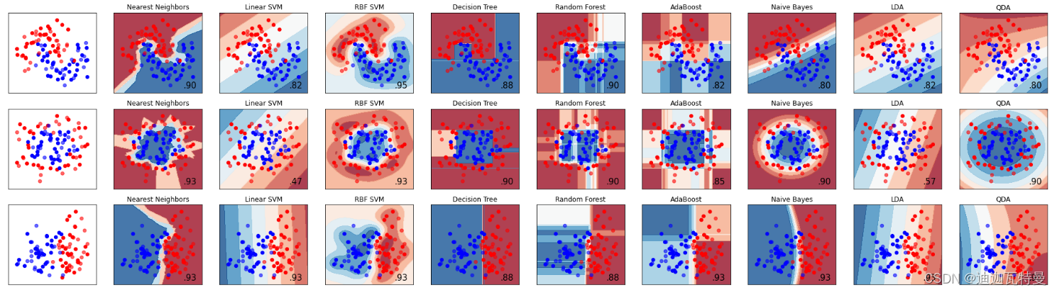
Here, three sample sets are randomly generated, and the split surfaces are approximately moon-shaped, circular and linear. We can focus on comparing the division of the sample space between decision trees and random forests:

1) It can be seen from the accuracy rate that the random forest is better than a single decision tree on the three test sets, 90%>88%, 90%=90%, 88%=88%;

2) It can be seen intuitively from the feature space that random forest has stronger segmentation ability (non-linear fitting ability) than decision tree.

6. Application direction of Random Forest